Sliding Window Inference in Large-Scale 3D Imaging Models
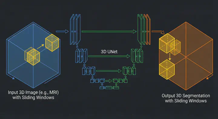 Illustration fo Sliding Window technique with 3D UNet
Table of Contents
I recently started working on a project involving a 3D whole-body imaging segmentation UNet. It was a foundational model, the kind that promises state-of-the-art results and robust performance across varied datasets. But it came with huge trouble for individuals like me using cloud environments (usually the free tier) to run those models, the model weights alone were approximately 14GB.
For anyone who has stared at the nvidia-smi output praying for free memory, you know where this is going.
I was working with a constrained setup with a 16GB VRAM GPU. The model alone, without accounting for the PyTorch and other packages overhead, immediately ate up about 16GB of VRAM. That left me with no VRAM to handle the input image, and the output prediction.
As you probably figured, I ran into the infamous CUDA out of memory.
In this post, I want to walk you through the solution to this memory bottleneck: the Sliding Window Inference technique. We will look at how tools like Patchly and MONAI implement this.
Sliding Window Inference
When you can’t process the whole image, you process parts of it. This is the core philosophy of the Sliding Window technique.
Instead of feeding the entire 3D volume into the GPU, we define a smaller “window”. We slide this window across the image, run inference on just that small chunk, store the prediction, and move to the next position. Once we’ve scanned the whole image, we stitch the predictions back together.
This solves the input memory problem. The GPU only ever “sees” a small tensor, regardless of how huge the original scan is.
In deep learning, specifically 3D medical imaging, this very technique is applied:
- Crop: We cut a sub-volume (a patch) from the original 3D image, let the path size be $96 \times 96 \times 96$ voxels.
- Infer: We feed just that patch into the GPU. Since the input is small, the activation maps are small, and the memory usage stays low.
- Place: We take the model’s output for that patch and place it into a blank “canvas” the size of the original image.
- Slide: We move the patch over by a defined step and repeat.
This sounds simple, but implementation details matter. That’s when I stumbled upon Patchly and MONAI.
Patchly
I first came across Patchly, a library developed by the folks at MIC-DKFZ (the German Cancer Research Center). They face these massive 3D volume problems daily, so their solution has been put to real tests.
Patchly separates the problem into two distinct workers: a Sampler and an Aggregator.
The Sampler is responsible for slicing the input image into a grid. The Sampler samples patches from the image in a grid-like manner as depicted in the image. What’s cool about Patchly is how it handles the image borders. If your image size isn’t perfectly divisible by your patch size, you have a problem at the border. Patchly offers multiple border-handling strategies. Squeeze sampling strategy (the default), where it slightly adjusts the step size of the final patches so they fit perfectly inside the image without going out of bounds or needing zero-padding.
](/post/sliding-window-inference/images/sampler_hue123761ae094a04acaece71ddf15c4a4_111056_0937121308a1ddf0399e6f9ef31dab16.webp)
Why Overlap Matters in Sampling
You might think the most efficient way is to cut the image into non-overlapping grids, like a chessboard. The problem with that is border artifacts.
Convolutional Neural Networks (CNNs) are generally confident in the center of their receptive field but “nervous” at the edges. Padding adds zeros or reflections that aren’t real data, making predictions at the patch borders unreliable. If you stitch non-overlapping patches, you will likely see visible grid lines in your output segmentation.
Patchly (and MONAI, as we will see later) solves this by overlapping the windows, usually by 25% or 50%. This means a voxel in the middle of the volume might be predicted 4 or 8 times by different passing windows. The Aggregator then has to decide how to combine these multiple predictions.
Aggregation and Gaussian Weighting
The simplest way to combine overlapping predictions is Average Aggregation: you just take the mean of all predictions for a specific voxel.
But Patchly offers a smarter mathematical approach: Gaussian Weighting.
The idea is that the model is most confident in the center of the patch and least confident at the edges. So, instead of a simple average, we apply a Gaussian kernel to the prediction patch before adding it to the final map.
Mathematically, for a voxel predicted by overlapping patches, the final value is: $$ V_{final}(x) = \frac{\sum_{i} P_i(x) \cdot G_i(x)}{\sum_{i} G_i(x)} $$
Where $P_i$ is the prediction from patch $i$, and $G_i$ is the weight from the Gaussian kernel (highest at the center, approaching zero at the edges).
This suppresses the edge artifacts almost entirely, resulting in a smooth, seamless segmentation map.
Chunk Aggregation: Solving the Output OOM
One specific feature in Patchly that caught my eye was Chunk Aggregation, it solves a problem that I haven’t paid attention to at first.
Usually, we worry about the input fitting in RAM. But in many scenarios as it the case 3D medical deep learning pipelines where the output is softmax predictions for different classes, the output can be the bottleneck. If you are predicting 100 classes for a $512 \times 512 \times 512$ volume, your output tensor is massive. Even if you infer patch-by-patch, if you try to hold the entire predicted volume in GPU memory to stitch it back together, you might hit OOM again.
Patchly’s Chunk Aggregation virtually divides the image into chunks that fit in memory. It samples and aggregates patches only for one chunk, finishes it, offloads it (or saves it), and then moves to the next. It’s a brilliant way to ensure that neither the forward pass nor the reconstruction blows up your RAM.
](/post/sliding-window-inference/images/chunk_hu11facf0320cd36ee8477d7f971611759_71125_3527524ec996cc109f4cde95e4273f10.webp)
Sliding Window Inference in MONAI
If you are already in the PyTorch ecosystem, you might prefer MONAI (Medical Open Network for AI). They implement this logic directly in the monai.inferers package.
MONAI provides sliding window inference in the monai.inferers package. It functions similar to Patchly but is optimized to work directly with PyTorch tensors and dictionaries and runs the forward pass for you inside the loop. While Patchly is designed for working with larger-than-memory N-dimensional images in a wider range of scenarios.
There are two ways to use it, depending on how you want to structure your code:
1. The Function: sliding_window_inference
It is a functional, stateless utility. You pass everything, the inputs, the window size, and your model (the predictor), in a single function call, and it runs the loop immediately.
from monai.inferers import sliding_window_inference

val_outputs = sliding_window_inference(
    inputs=val_images,
    roi_size=(96, 96, 96),
    sw_batch_size=4,
    predictor=model,
    overlap=0.25,
    mode="gaussian"
)
Ideal for simple scripts or direct application on a tensor. You can use this when you are writing a standard, custom PyTorch training loop (e.g., for batch in val_loader:). Since you control the loop, it’s easier to just call the function explicitly. It’s also much better for debugging because all your parameters are right there in front of you, not hidden inside an object defined in another file.
2. The Class: SlidingWindowInferer
It is a class-based, stateful object, that needs to be initialized beforehand. You define the window size and batch size when you create the object, not when you run the data.
from monai.inferers import SlidingWindowInferer

# Define the settings once (e.g., in a config or setup block)
inferer = SlidingWindowInferer(
    roi_size=(96, 96, 96),
    sw_batch_size=4,
    overlap=0.25,
    mode="gaussian"
)

# Use it later. The code running this doesn't need to know the window size.
val_outputs = inferer(inputs=val_images, network=model)
Best for structured pipelines where you define an inferer once and use it across. And also comes in handy when you want to experiment with different inferers. Use this if you are building a larger system or using MONAI’s high-level engines like SupervisedEvaluator. In these systems, the training engine expects a generic “inferer” object to handle the work. It doesn’t want to know about your window sizes or overlap; it just wants to call inferer(). This is also the standard way to do things if you are using MONAI Bundles or loading your training configuration from a YAML/JSON file.
An important parameter here is sw_batch_size.This isn’t the training batch size; it’s how many windows the GPU processes in parallel. If your GPU has space, you can process 4 windows at once, this speeds up inference significantly if you have some VRAM headroom.
MONAI also supports mode="gaussian" out of the box, handling that blending math we discussed earlier.
While MONAI is incredibly convenient, it typically allocates the full output tensor in memory at the start. If your output is 30GB, MONAI might still crash your RAM, whereas Patchly’s chunking would survive.
Worked Examples
Nothing beats learning from worked examples and reading code yourself. To help you do just that, here are some interesting examples of models using the sliding window technique in 3D medical imaging:
- SegResNet for 3D Brain Tumor Segmentation
- UNet for 3D Spleen Segmentation
- Swin UNETR for 3D Brain Tumor Segmentation
- UNETR for 3D Multi-organ Segmentation
Conclusion
If you are dealing with massive 3D medical models, don’t let the OOM error stop you.
- Sliding Window is the standard solution to decouple input size from memory limits.
- Overlap and Gaussian blending are mandatory to avoid artifacts.
- Patchly is amazing for N-dimensional images enabling inference and other processing steps on extremely large images under different scenarios.
- MONAI offers the smoothest integration for PyTorch workflows.